Tutorial
Getting the tutorial data and setting up
This notebook demonstrates how to use scATAcat, a tool designed for annotationg cell-types in scATAC-seq data.
The necessary data to run the code provided below can be found here. Please download the data and ensure it is stored in a folder named data.
Load the libraries
import pickle
import pandas as pd
import sklearn
import numpy as np
import scanpy as sc
import scipy.sparse
import anndata
import matplotlib.pylab as plt
from sklearn.decomposition import PCA
import copy
import logging as logg
from sklearn import preprocessing
import os
import warnings
import scATAcat
import seaborn as sns
import random as rn

warnings.filterwarnings('ignore')
Set seed for reproducibility
sd = 1234
np.random.seed(sd)
rn.seed(sd)
%env PYTHONHASHSEED=0
env: PYTHONHASHSEED=0
define necessary parameters
results_dir = "./results"
output_dir = results_dir + "/outputs/"
figures_dir = results_dir + "/figures/"
data_dir = "./data/"

for dir in [figures_dir, output_dir]:
    if not os.path.exists(dir):
        os.makedirs(dir)
0 - Load scATAC-seq data
Here we load the scATAC-seq data from Buenrostro et al., 2018. This datset comprises of 2,210 cells human hematopoietic progenitor cells which are obtained from bone marrow and isolated via fluorescence-activated cell sorting (FACS). FACS enables sorting of single cells into a well plate using cell-type specific cell-surface markers and thereby provides a true cell-type annotation for each cell in the data. This means, we know the real cell-type identities of this cells.
Here, ENCODE
cCREs are used as
the reference frame/features. We calculated the cCRE coverages for each
cell, which is provided in data/matrix_sparse.pkl. The column and
index IDs of this matrix are given in data/cell_IDs.csv and
features.csv, respectively.
ENCODE_coverage_per_cell_df= pickle.load(open(data_dir + 'matrix_sparse.pkl','rb'))
ENCODE_coverage_per_cell_df
<926535x2210 sparse matrix of type '<class 'numpy.float32'>'
    with 18562502 stored elements in Compressed Sparse Row format>
ENCODE_cCREs = pd.read_csv(data_dir +"features.csv", index_col=0)
ENCODE_cCREs.index.name = None
ENCODE_cCREs.columns = ['cCREs']
ENCODE_cCREs.head()
| cCREs | |
|---|---|
| chr1_181251_181601 | chr1_181251_181601 |
| chr1_190865_191071 | chr1_190865_191071 |
| chr1_778562_778912 | chr1_778562_778912 |
| chr1_779086_779355 | chr1_779086_779355 |
| chr1_779727_780060 | chr1_779727_780060 |
cell_IDs = pd.read_csv(data_dir +"cell_IDs.csv", index_col=0)
cell_IDs.index.name = None
cell_IDs.columns = ['cell_IDs']
cell_IDs.head()
| cell_IDs | |
|---|---|
| CLP_0 | CLP_0 |
| CLP_1 | CLP_1 |
| CMP_0 | CMP_0 |
| CMP_1 | CMP_1 |
| CMP_2 | CMP_2 |
1 - initialize the AnnData object
scATAcat relies on AnnData package when working with datasets. Here we define an AnnData object from our scATAC-seq data. Note that AmnnData requires observations as the columns and variables as indexes. We use csr matrix format.
sc_completeFeatures_adata = anndata.AnnData(ENCODE_coverage_per_cell_df.transpose().tocsr(), var=ENCODE_cCREs, obs=cell_IDs)
sc_completeFeatures_adata
AnnData object with n_obs × n_vars = 2210 × 926535
    obs: 'cell_IDs'
    var: 'cCREs'
2 - add binary layer to AnnData
We binarize the matrix to enable further processing and filtering. This new matrix is added as a new layer to our AnnData object with the keyword “binary”.
scATAcat.add_binary_layer(sc_completeFeatures_adata, binary_layer_key="binary")
AnnData object with n_obs × n_vars = 2210 × 926535
    obs: 'cell_IDs'
    var: 'cCREs'
    layers: 'binary'
3- calculate & plot cell and feature statistics
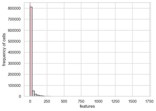
cell_feature_statistics() function calculates the quality features
like “number of features per cell” and “number of cells per feature”.
plot_feature_statistics() and plot_cell_statistics() functions
enables viuzalizations of these quality features.
scATAcat.cell_feature_statistics(sc_completeFeatures_adata, binary_layer_key ='binary')
AnnData object with n_obs × n_vars = 2210 × 926535
    obs: 'cell_IDs'
    var: 'cCREs'
    obsm: 'num_feature_per_cell'
    varm: 'num_cell_per_feature'
    layers: 'binary'
scATAcat.plot_feature_statistics(sc_completeFeatures_adata, threshold=3, bins=50, color="lightgrey", save=True, save_dir = figures_dir +"/feature_statistics_plot.png")
AnnData object with n_obs × n_vars = 2210 × 926535
    obs: 'cell_IDs'
    var: 'cCREs'
    obsm: 'num_feature_per_cell'
    varm: 'num_cell_per_feature'
    layers: 'binary'
scATAcat.plot_cell_statistics(sc_completeFeatures_adata, threshold=1000, bins=50, color="lightgrey", save=True, save_dir = figures_dir + "/cell_statistics_plot.png")
AnnData object with n_obs × n_vars = 2210 × 926535
    obs: 'cell_IDs'
    var: 'cCREs'
    obsm: 'num_feature_per_cell'
    varm: 'num_cell_per_feature'
    layers: 'binary'
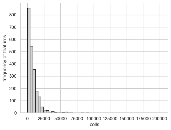
4- filter the cells and features
preproces_sc_matrix() function is used to filter unwanted cells and
features. By default, eatures which occur in less than
feature_cutoff=3 cells get eliminated. In the level of cells, we
filter out cells with fewer than feature_cutoff=1000 and more than
cell_cutoff_max=80000 non-zero features. Additionally, we get rid of
the features within Y chromosome to avoid gender biases, controlled by
remove_chrY = True paramater.
sc_completeFeatures_adata
AnnData object with n_obs × n_vars = 2210 × 926535
    obs: 'cell_IDs'
    var: 'cCREs'
    obsm: 'num_feature_per_cell'
    varm: 'num_cell_per_feature'
    layers: 'binary'
sc_filteredFeatures_adata = scATAcat.preproces_sc_matrix(sc_completeFeatures_adata,cell_cutoff=1000,cell_cutoff_max=80000, feature_cutoff=3, remove_chrY = True, var_key = 'cCREs', copy=True)
sc_filteredFeatures_adata
View of AnnData object with n_obs × n_vars = 1872 × 501699
    obs: 'cell_IDs'
    var: 'cCREs'
    obsm: 'num_feature_per_cell'
    varm: 'num_cell_per_feature'
    layers: 'binary'
note that here we filtered almost half of the features!
5- load & preprocess the bulk data
scATAcat requires bulk prototype data to provide cell-type annotation
for query scATAC-seq data. For this tutorial, we use prototype
cell-types derived from bulk ATAC-seq data of hematopoietic progenitors
from Corces et al., 2016.
This dataset comprises of bulk ATAC-seq data of hematopoietic
progenitors, serving as an perfect example for our purposes. An AnnData
object containing this dataset can easily be generated using the
generate_bulk_sparse_AnnData() function, which prepares the data in
a format suitable for scATAcat analysis. data/bulk_prototypes.pkl
matrix includes the cCRE coverages of each bulk sample.
bulk_by_ENCODE_peaks_df_annotated = pickle.load(open(data_dir + 'bulk_prototypes.pkl','rb'))
bulk_completeFeatures_adata = scATAcat.generate_bulk_sparse_AnnData(bulk_by_ENCODE_peaks_df_annotated)
bulk_completeFeatures_adata
AnnData object with n_obs × n_vars = 43 × 926535
    obs: 'cell_types'
    var: 'cCREs'
preprocess_bulk_adata() function preprocesses prototype/bulk AnnData
by optionally removing features associated with chromosome Y, controlled
by remove_chrY = True paramater.
bulk_completeFeatures_adata = scATAcat.preprocess_bulk_adata(bulk_completeFeatures_adata, remove_chrY=True, var_key = 'cCREs', copy=False)
6 - Overlap bulk and sc features
Before we proceed with our analysis, it’s essential to align the
features between the bulk and single-cell (sc) AnnData objects. Although
we initially used the same set of candidate cis-regulatory elements
(cCREs), different filtering criteria applied to the bulk and sc data
may have resulted in discrepancies. A unified feature set is crucial for
integrating these datasets effectively. We define the common variables
with overlap_vars() function and subset both the AnnData objects to
these common variables using subset_adata_vars() function.
sc_bulk_common_vars = scATAcat.overlap_vars(sc_filteredFeatures_adata, bulk_completeFeatures_adata)
len(sc_bulk_common_vars)
501699
sc_commonFeatures_adata = scATAcat.subset_adata_vars(sc_filteredFeatures_adata, vars_list=sc_bulk_common_vars, copy_=True)
bulk_commonFeatures_adata = scATAcat.subset_adata_vars(bulk_completeFeatures_adata, vars_list=sc_bulk_common_vars, copy_=True)
7- doublet removal
If you’ve applied a doublet detection algorithm, this is a good place to remove these cells from your analysis. In our case, removal isn’t necessary as our data was obtained from sorted individual cells. However, we strongly recommend removing doublets from the analysis, as these cells can significantly impact downstream analysis. We have used AMULET and have achieved good results with it.
8- apply TF-IDF
We continue with processign our sc data. We apply TF-logIDF normalization. This results in re-weighted features (cCREs) by assigning greater weight to more important features.
scATAcat.apply_TFIDF_sparse(sc_commonFeatures_adata, binary_layer_key='binary', TFIDF_key='TF_logIDF' )
AnnData object with n_obs × n_vars = 1872 × 501699
    obs: 'cell_IDs'
    var: 'cCREs'
    obsm: 'num_feature_per_cell'
    varm: 'num_cell_per_feature'
    layers: 'binary', 'TF_logIDF'
9 - subset matrices to differential cCREs
Next, we subset the data to focus on the differential cCREs as defined
by the reference bulk ATAC-seq data. These regions are identified using
the DiffBind R package (version 3.0) by conducting pairwise comparisons
between each cell type. The file data/differential_features.csv
contains the union of the top 2000 differential cCREs from each
comparison
We next subset both the sc and bulk AnnData objects to these differential regions with the assumption that these specific cCREs contain the most discriminative information and are indicative of cell-type specificity.
pairwise_top2000_cCREs = pd.read_table(data_dir +'/differential_features.csv',delimiter="\t",header=None)

pairwise_top2000_cCREs.head()
| 0 | |
|---|---|
| 0 | chr1_1842820_1843169 |
| 1 | chr1_1895700_1895891 |
| 2 | chr1_1895944_1896292 |
| 3 | chr1_1966481_1966686 |
| 4 | chr1_2045674_2045954 |
len(pairwise_top2000_cCREs)
21034
common_differential_vars = list(set(list(sc_bulk_common_vars)) & set(list(pairwise_top2000_cCREs[0].tolist())))

len(common_differential_vars)
19412
bulk_commonDiffFeatures_adata = scATAcat.subset_adata_vars(bulk_commonFeatures_adata,
                                                 vars_list=common_differential_vars,
                                                 copy_=True)
sc_commonDiffFeatures_adata = scATAcat.subset_adata_vars(sc_commonFeatures_adata,
                                                 vars_list=common_differential_vars,
                                                 copy_=True)
10- dimention reduction and clustering
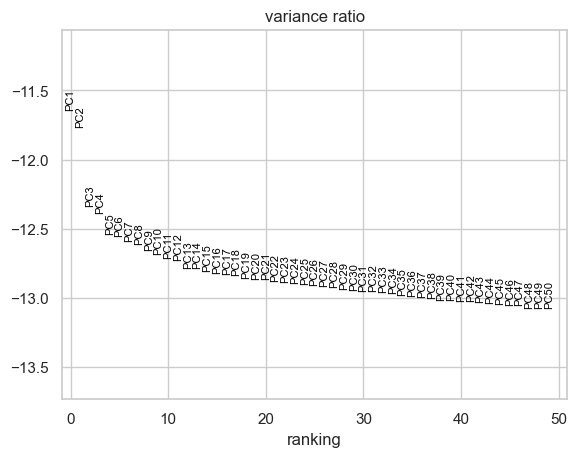
The next step is dimension reduction. We apply principal component
analysis (PCA) using apply_PCA() function. Sometimes the first
principal component may capture the variation in the sequencing depth
among among cells rather than biological variation. In such instances,
it might be advisable to exclude the first PC. Below, we examine whether
there is such an association.
scATAcat.apply_PCA(sc_commonDiffFeatures_adata, layer_key ='TF_logIDF', svd_solver='arpack', random_state=0)
AnnData object with n_obs × n_vars = 1872 × 19412
    obs: 'cell_IDs'
    var: 'cCREs'
    uns: 'pca'
    obsm: 'num_feature_per_cell', 'X_pca'
    varm: 'num_cell_per_feature', 'PCs'
    layers: 'binary', 'TF_logIDF'
with plt.rc_context():
    sc.pl.pca_variance_ratio(sc_commonDiffFeatures_adata, n_pcs=50, log=True, show=False)
    plt.savefig(figures_dir + "/pca_variance_ratio.pdf", bbox_inches="tight")
seqDepth_PC1_plot = sns.jointplot(
    x=sc_commonDiffFeatures_adata.obsm['X_pca'][:,0],
    y=np.sqrt(sc_commonDiffFeatures_adata.obsm['num_feature_per_cell']),
    kind="kde",fill=True
)

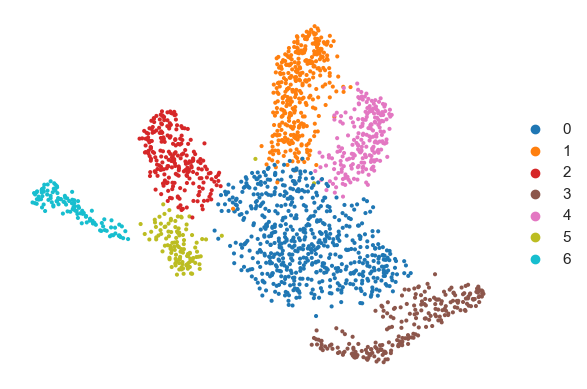
11 - apply UMAP & leiden clustering
Next, we compute the nearest neighbors and apply Leiden clustering. These clusters are then visualized in a low-dimensional UMAP embedding. Note that we these funtions are borrowed from ScanPy package.
sc.pp.neighbors(sc_commonDiffFeatures_adata, n_pcs = 50, n_neighbors = 30, random_state=0)
leiden_resolution=0.4
leiden_key="leiden_"+ str(leiden_resolution)
sc.tl.umap(sc_commonDiffFeatures_adata, random_state=0)
sc.tl.leiden(sc_commonDiffFeatures_adata, resolution=leiden_resolution,key_added=leiden_key, random_state=0)
# one can explicity specify the colors of their liking
sc_commonDiffFeatures_adata.uns[leiden_key +'_colors'] = ['#1f77b4',
'#ff7f0e',
'#d62728',
'#8c564b',
'#e377c2',
'#bcbd22',
'#17becf',
'#2ca02c']
with plt.rc_context():
    sc.pl.umap(sc_commonDiffFeatures_adata, color=leiden_key, show=False,size=35 , add_outline=False, frameon=False, title="")
    plt.savefig(figures_dir + "/"+ leiden_key+ ".pdf", bbox_inches="tight")
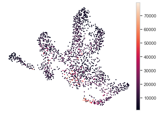
We can also examine the sequencing depth of cells to determine if it impacts the clustering results:
sc_commonDiffFeatures_adata.obs['num_feature_per_cell_'] = sc_commonDiffFeatures_adata.obsm['num_feature_per_cell']
with plt.rc_context():
    sc.pl.umap(sc_commonDiffFeatures_adata, color='num_feature_per_cell_', add_outline=False, frameon=False,title ="", save=False, size=25 )
    plt.savefig(figures_dir + "/seq_depth_umap.pdf", bbox_inches="tight")
<Figure size 640x480 with 0 Axes>
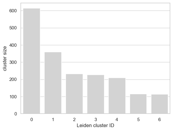
12 - create pseudobulks according to the cluster assignments
We form pseudobulks by aggregating the cells in each cluster.
get_pseudobulk_matrix_ext() function is used to obtain pseudobulk
matrix and generate_bulk_sparse_AnnData() is repurposed to generate
an AnnData object for the pseudobulks. Note that the pseudobulk matrix
has the common cCREs as variables.
cell_cluster_assignments = pd.DataFrame(sc_commonDiffFeatures_adata.obs[leiden_key].copy())
cell_cluster_assignments
| leiden_0.4 | |
|---|---|
| CLP_1 | 6 |
| CMP_0 | 0 |
| CMP_1 | 0 |
| CMP_2 | 0 |
| CMP_3 | 3 |
| ... | ... |
| LMPP_90 | 5 |
| LMPP_91 | 5 |
| LMPP_93 | 5 |
| LMPP_94 | 5 |
| LMPP_95 | 5 |
1872 rows × 1 columns
cell_cluster_sizes = pd.DataFrame(cell_cluster_assignments[leiden_key].value_counts())
cell_cluster_sizes['leiden_clusters'] = cell_cluster_sizes.index
cell_cluster_sizes.head()
| count | leiden_clusters | |
|---|---|---|
| leiden_0.4 | ||
| 0 | 614 | 0 |
| 1 | 359 | 1 |
| 2 | 233 | 2 |
| 3 | 227 | 3 |
| 4 | 210 | 4 |
for clust_id in set(sc_commonDiffFeatures_adata.obs[leiden_key].values):
    clust_df= sc_commonDiffFeatures_adata[sc_commonDiffFeatures_adata.obs[leiden_key]==clust_id]
cell_types = ([(r.split('_')[0]) for r in clust_df.obs[leiden_key].index])
# plot a bar chart
sns.set_style("whitegrid")
ax= sns.barplot(
    y="count",
    x="leiden_clusters",
    data=cell_cluster_sizes,
    color='lightgrey');
ax.yaxis.grid(True,color="lightgrey")
ax.axes.set_xlabel("Leiden cluster ID")
ax.axes.set_ylabel("cluster size")
#atickt(yticks=(list(range(0,1500,100))))
plt.savefig(figures_dir + "/cluster_sizes_"+leiden_key+".pdf", dpi=250)
13 - Coembedding prototypes with pseudobulks in PCA space
We preprocess both the bulk and pseudobulk data prior to co-embedding.
First, we apply library size normalization and log2 transformation to
the datasets using the preprocessing_libsize_norm_log2() function,
then subset the matrices to include only differential cCREs.
Next, we perform z-normalization using the
preprocessing_standardization() function. This function can also
accept external parameters for standard deviation (std_) and mean
(mean_). When normalizing the pseudobulk matrix, we utilize the
std_ and mean_ values from the bulk AnnData to facilitate the
integration of these datasets.
Processing
pseudobulk_commonFeatures_adata = scATAcat.generate_bulk_sparse_AnnData(scATAcat.get_pseudobulk_matrix_ext(adata_to_subset=sc_commonFeatures_adata, adata_to_get_clusters=sc_commonDiffFeatures_adata, cluster_key=leiden_key, method = 'sum'))
pseudobulk_commonFeatures_adata
AnnData object with n_obs × n_vars = 7 × 501699
    obs: 'cell_types'
    var: 'cCREs'
scATAcat.preprocessing_libsize_norm_log2(pseudobulk_commonFeatures_adata)
AnnData object with n_obs × n_vars = 7 × 501699
    obs: 'cell_types'
    var: 'cCREs'
    layers: 'libsize_norm_log2'
scATAcat.preprocessing_libsize_norm_log2(bulk_commonFeatures_adata)
AnnData object with n_obs × n_vars = 43 × 501699
    obs: 'cell_types'
    var: 'cCREs'
    layers: 'libsize_norm_log2'
bulk_commonDiffFeatures_adata = scATAcat.subset_adata_vars(bulk_commonFeatures_adata,
                                                 vars_list=common_differential_vars,
                                                 copy_=True)
bulk_commonDiffFeatures_adata
AnnData object with n_obs × n_vars = 43 × 19412
    obs: 'cell_types'
    var: 'cCREs'
    layers: 'libsize_norm_log2'
pseudobulk_commonDiffFeatures_adata = scATAcat.subset_adata_vars(pseudobulk_commonFeatures_adata,
                                                 vars_list=common_differential_vars,
                                                 copy_=True)
scATAcat.preprocessing_standardization(bulk_commonDiffFeatures_adata, input_layer_key="libsize_norm_log2", zero_center=True)
adding std with default keywords
adding mean with default keywords
AnnData object with n_obs × n_vars = 43 × 19412
    obs: 'cell_types'
    var: 'cCREs', 'feature_std', 'feature_mean'
    layers: 'libsize_norm_log2', 'libsize_norm_log2_std'
bulk_commonDiffFeatures_adata
AnnData object with n_obs × n_vars = 43 × 19412
    obs: 'cell_types'
    var: 'cCREs', 'feature_std', 'feature_mean'
    layers: 'libsize_norm_log2', 'libsize_norm_log2_std'
scATAcat.preprocessing_standardization(pseudobulk_commonDiffFeatures_adata, input_layer_key="libsize_norm_log2", zero_center=False,
                              output_layer_key= "libsize_norm_log2_bulk_scaled_diff",
                              std_key= None,  mean_key=None,
                              std_ = bulk_commonDiffFeatures_adata.var["feature_std"],
                              mean_= bulk_commonDiffFeatures_adata.var["feature_mean"])
adding std with default keywords
adding mean with default keywords
AnnData object with n_obs × n_vars = 7 × 19412
    obs: 'cell_types'
    var: 'cCREs', 'feature_std', 'feature_mean'
    layers: 'libsize_norm_log2', 'libsize_norm_log2_bulk_scaled_diff'
## as an option, I can add the color codes from the clustering/ sc adata as a paramater for the pseudobulk matrix
leiden_color_key = leiden_key+"_colors"
pseudobulk_commonDiffFeatures_adata.uns[leiden_color_key] = sc_commonDiffFeatures_adata.uns[leiden_color_key]
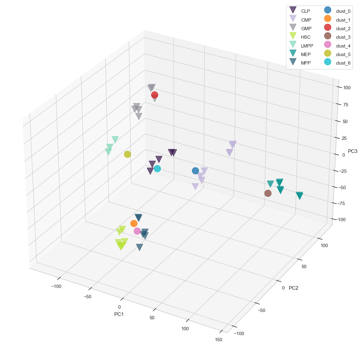
Projection
Finally, we co-embed the bulk prototypes together with the pseudobulks using the projection() function. This function provides highly customizable visualization options, some of which are provided below
## as an option, one can add the color codes from the clustering of sc adata as a paramater for the pseudobulk matrix
leiden_color_key = leiden_key+"_colors"
pseudobulk_commonDiffFeatures_adata.uns[leiden_color_key] = sc_commonDiffFeatures_adata.uns[leiden_color_key]
result= scATAcat.projection(prototype_adata=bulk_commonDiffFeatures_adata, pseudobulk_adata=pseudobulk_commonDiffFeatures_adata, prototype_layer_key = "libsize_norm_log2_std", pseudobulk_layer_key="libsize_norm_log2_bulk_scaled_diff", color_key=leiden_color_key, pseudobulk_label_font_size =13, prototype_label_font_size = 0,
prototype_colors = ['#38184C',  "#BDB0D9", "#92929C","#BAE33A", "#7ED9B7", "#008F8C", "#275974"], pseudobulk_colors =  None, pseudobulk_point_size=250, prototype_point_size=250, pseudobulk_point_alpha=0.8, prototype_point_alpha=0.7, cmap='twilight_shifted', prototype_legend = True, pseudobulk_legend = True, save_path = figures_dir + "projection.png")

result_noLabel = scATAcat.projection(prototype_adata=bulk_commonDiffFeatures_adata, pseudobulk_adata=pseudobulk_commonDiffFeatures_adata, prototype_layer_key = "libsize_norm_log2_std", pseudobulk_layer_key="libsize_norm_log2_bulk_scaled_diff", color_key=leiden_color_key, pseudobulk_label_font_size =0, prototype_label_font_size =0,
                            prototype_colors = ['#38184C',  "#BDB0D9", "#92929C","#BAE33A", "#7ED9B7", "#008F8C", "#275974"], pseudobulk_colors =  None, pseudobulk_point_size=250, prototype_point_size=250, pseudobulk_point_alpha=0.8, prototype_point_alpha=0.7, cmap='twilight_shifted', prototype_legend = True, pseudobulk_legend = True, save_path = figures_dir + "projection_noLabel.png")
result_noLabel_noLegend = scATAcat.projection(prototype_adata=bulk_commonDiffFeatures_adata, pseudobulk_adata=pseudobulk_commonDiffFeatures_adata, prototype_layer_key = "libsize_norm_log2_std", pseudobulk_layer_key="libsize_norm_log2_bulk_scaled_diff", color_key=leiden_color_key, pseudobulk_label_font_size =0, prototype_label_font_size =0,
                            prototype_colors = ['#38184C',  "#BDB0D9", "#92929C","#BAE33A", "#7ED9B7", "#008F8C", "#275974"], pseudobulk_colors =  None, pseudobulk_point_size=250, prototype_point_size=250, pseudobulk_point_alpha=0.8, prototype_point_alpha=0.7, cmap='twilight_shifted', prototype_legend = False, pseudobulk_legend = False, save_path = figures_dir + "projection_noLabel_noLegend.png", fig_size_inches=(15,15))

result_noLabel_noLegend = scATAcat.projection(prototype_adata=bulk_commonDiffFeatures_adata, pseudobulk_adata=pseudobulk_commonDiffFeatures_adata, prototype_layer_key = "libsize_norm_log2_std", pseudobulk_layer_key="libsize_norm_log2_bulk_scaled_diff", color_key=leiden_color_key, pseudobulk_label_font_size =0, prototype_label_font_size =0,
                            prototype_colors = ['#38184C',  "#BDB0D9", "#92929C","#BAE33A", "#7ED9B7", "#008F8C", "#275974"], pseudobulk_colors =  None, pseudobulk_point_size=250, prototype_point_size=250, pseudobulk_point_alpha=0.8, prototype_point_alpha=0.7, cmap='twilight_shifted', prototype_legend = False, pseudobulk_legend = False, save_path = figures_dir + "projection_noLabel_noLegend.pdf", fig_size_inches=(15,15))
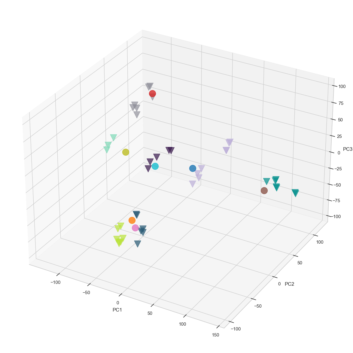
14 - Determining the cluster annotations by matching Clusters to Prototypes
Co-embedding protoypes with pseudobulks, and visualizing the projection in 3D PCA space facilitates a simplified interpretation of cell-type relationships. However, determining the annotations solely based on a visualisation may be tedious. In particular, the first three PCs used in the projection might not suffice to fully capture the inherent structure of the high dimensional data. Following common practice, we therefore keep a larger number of dimension (typically 30 if there are enough samples available) to compute Euclidean distances in this high-dimensional embedding space.
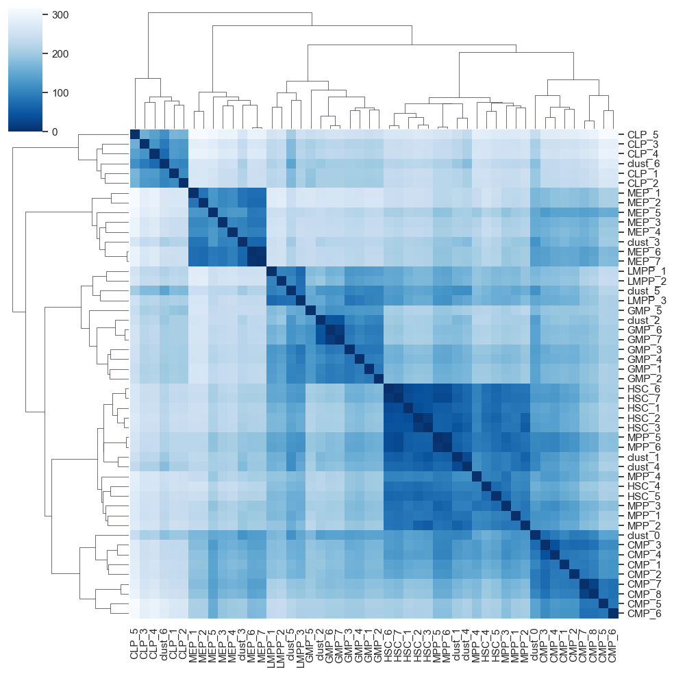
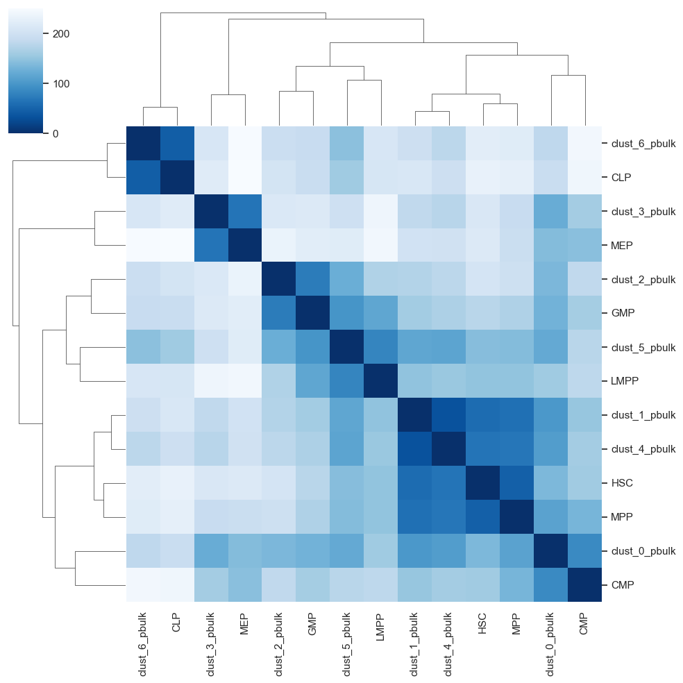
To obtain a matching between pseudobulk clusters and prototype samples, we first compute centroids for each of the prototype cell-types. Next, we compute the Euclidean distances (in many dimensions) between the pseudobulk clusters and the centroids, yielding a matrix vizualized in heatmap. Finally, we annotate each pseudobulk cluster by its closest centroid of a cell-type.
Below, we provide various data visualization options that are useful for interpreting the relationships between pseudobulks and prototypes
heatmap = scATAcat.plot_pca_dist_heatmap(result[1],result[2])
centroid_heatmap = scATAcat.plot_pca_dist_cent_heatmap(result[1],result[2])
heatmap[0].savefig(figures_dir +"/heatmap.png")
centroid_heatmap[0].savefig(figures_dir +"/centroid_heatmap.png")
clusterID_prediction_dict = scATAcat.get_closest_prototype_to_pseudobulk(centroid_heatmap[1])
clusterID_prediction_dict
{'clust_0_pbulk': 'CMP',
 'clust_1_pbulk': 'HSC',
 'clust_2_pbulk': 'GMP',
 'clust_3_pbulk': 'MEP',
 'clust_4_pbulk': 'HSC',
 'clust_5_pbulk': 'LMPP',
 'clust_6_pbulk': 'CLP'}
cluster_to_pseudobulk_heatmap_plot = sns.clustermap(scATAcat.get_pseudobulk_to_prototype_distance(centroid_heatmap[1], pbulk_to_prototype=True).T,yticklabels=True,xticklabels=True, cmap="Blues")
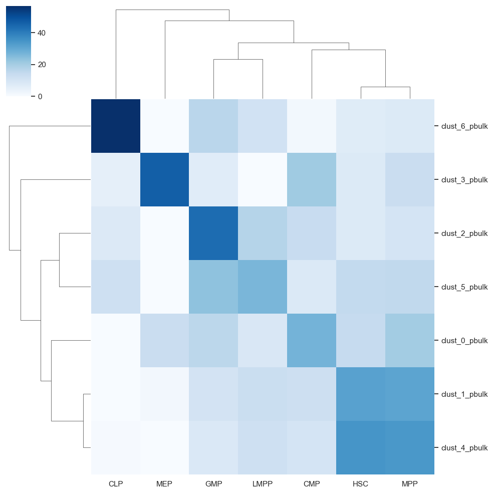
cluster_to_pseudobulk_heatmap_plot.savefig(figures_dir+"/cluster_to_pseudobulk_heatmap_plot.png")
# save vestor friendly pdf file
import matplotlib as mpl
mpl.rcParams['pdf.fonttype'] = 42
mpl.rcParams['ps.fonttype'] = 42

cluster_to_pseudobulk_heatmap_plot.savefig(figures_dir+"/cluster_to_pseudobulk_heatmap_plot.pdf")
15 - make a final dataframe including the cluster IDs and the final annotations of each cell:
cell_cluster_assignments
| leiden_0.4 | |
|---|---|
| CLP_1 | 6 |
| CMP_0 | 0 |
| CMP_1 | 0 |
| CMP_2 | 0 |
| CMP_3 | 3 |
| ... | ... |
| LMPP_90 | 5 |
| LMPP_91 | 5 |
| LMPP_93 | 5 |
| LMPP_94 | 5 |
| LMPP_95 | 5 |
1872 rows × 1 columns
modified_dict = {key.replace('clust_', '').replace('_pbulk', ''): value for key, value in clusterID_prediction_dict.items()}

print(modified_dict)
{'0': 'CMP', '1': 'HSC', '2': 'GMP', '3': 'MEP', '4': 'HSC', '5': 'LMPP', '6': 'CLP'}
# Convert cluster IDs to string if they are not already, to match the dictionary keys
cell_cluster_assignments['leiden_0.4'] = cell_cluster_assignments['leiden_0.4'].astype(str)

# Add a new column by mapping the 'ID' column to the modified_dict
cell_cluster_assignments['Annotation'] = cell_cluster_assignments['leiden_0.4'].map(modified_dict)

cell_cluster_assignments
| leiden_0.4 | Annotation | |
|---|---|---|
| CLP_1 | 6 | CLP |
| CMP_0 | 0 | CMP |
| CMP_1 | 0 | CMP |
| CMP_2 | 0 | CMP |
| CMP_3 | 3 | MEP |
| ... | ... | ... |
| LMPP_90 | 5 | LMPP |
| LMPP_91 | 5 | LMPP |
| LMPP_93 | 5 | LMPP |
| LMPP_94 | 5 | LMPP |
| LMPP_95 | 5 | LMPP |
1872 rows × 2 columns
cell_cluster_assignments.to_csv(output_dir +"cell_cluster_assignments.csv")
export AnnData object
- with open(output_dir +’/sc_commonDiffFeatures_adata.pkl’, ‘wb’) as f:
pickle.dump(sc_commonDiffFeatures_adata, f)